Free of shape priors
A polynomial can only bend the way its degree allows. Amp glow in one corner plus a diagonal gradient is already too much for it. MEMBRANE has no preferred shape, so it follows whatever your sky actually did.
The stiffest surface that still honours the sky.
A background model that removes light pollution, sky glow and vignetting from your frames without flattening the nebulosity you spent the night collecting. Runs inside Siril, on the image you already have open.
Every other background extractor asks the same question: which formula best passes through my sky samples? MEMBRANE asks a different one. It stretches an elastic sheet across the frame and lets the sky samples pull on it, then finds the shape where the sheet stops moving. Nothing forces it into a polynomial, and nothing lets it wobble between samples.
A polynomial can only bend the way its degree allows. Amp glow in one corner plus a diagonal gradient is already too much for it. MEMBRANE has no preferred shape, so it follows whatever your sky actually did.
Spline methods solve a dense system that grows with the cube of the sample count, so a fine sampling grid becomes painful. MEMBRANE solves coarse-to-fine on a pyramid; its cost tracks the grid, not the samples.
Where an object is masked out, the sheet simply spans the hole instead of extrapolating into it. That is why bright targets come out with their signal intact rather than sitting in a subtracted bowl.
1.0 rejected a sky sample by comparing it to a plane fitted across the whole frame, so any real curvature in the light pollution looked like an object and was thrown away. 1.1 compares each sample to its own neighbourhood instead, then re-weights the fit against its own residual so bright targets lose their vote without bright sky losing it too.
Rejection now runs against a robust local trend of the tile field, not a global plane. A bright corner, an off-frame moon or an airglow band stays in the model instead of being discarded as contamination.
The surface is solved, then every cell sitting above it is demoted and the surface is solved again. A cell below the surface keeps its vote, because that is noise, not nebulosity. Nothing is ever silenced completely, so genuinely bright sky can still bend the sheet.
The relaxation used to be forced flat exactly at the frame border, and a real gradient is not flat there. The solve now runs on a grid that extends past the image, so the fit keeps its slope right to the edge.
| Model | Time | Residual sky | Edge bias | Target signal kept |
|---|---|---|---|---|
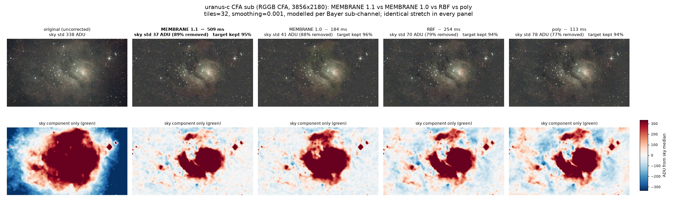
| MEMBRANE 1.1 | 509 ms | 36.9 ADU | -0.28 σ | 94.9% |
| MEMBRANE 1.0 | 184 ms | 40.5 ADU | -0.34 σ | 95.9% |
| RBF (thin-plate spline) | 254 ms | 70.1 ADU | -0.28 σ | 94.0% |
| Polynomial (degree 4) | 113 ms | 78.3 ADU | -0.24 σ | 93.7% |
M8, the single 120 s CFA sub, modelled per Bayer sub-channel. Uncorrected sky spread 338 ADU, uncorrected edge bias −0.90 σ. Residual sky is the spread of the robust tile sky levels with target tiles excluded, so a model cannot score well here by eating the nebula: that shows up in the last column instead.
| Model | Time | Residual sky | Edge bias | Target signal kept |
|---|---|---|---|---|
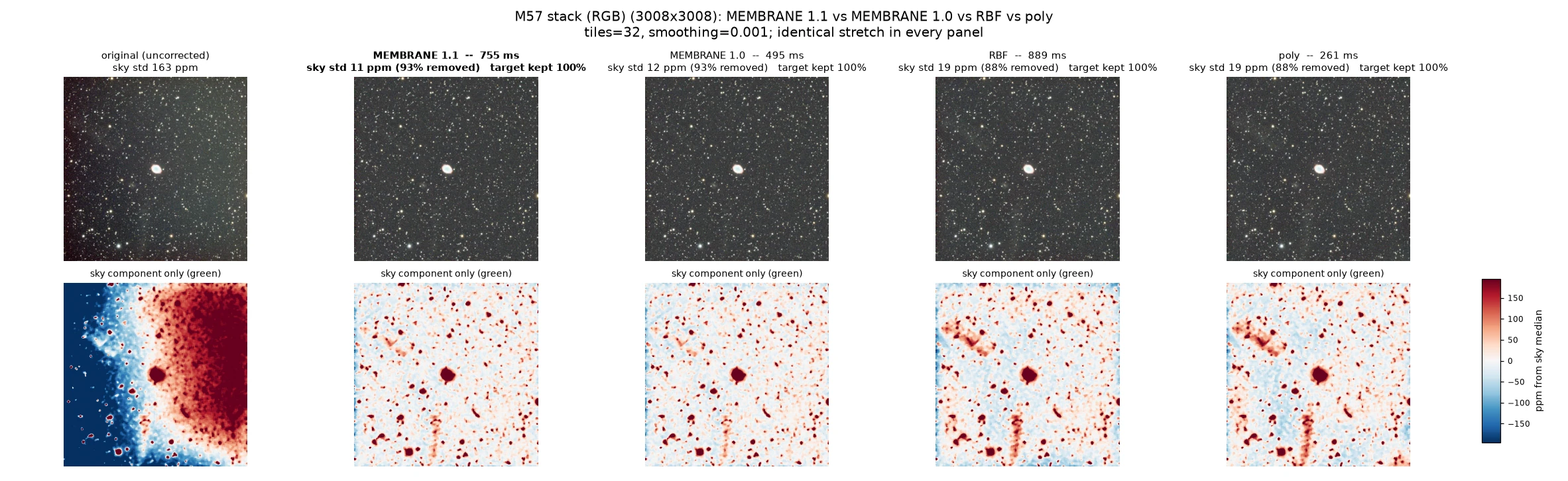
| MEMBRANE 1.1 | 755 ms | 10.7 ppm | 0.00 σ | 100.1% |
| MEMBRANE 1.0 | 495 ms | 11.9 ppm | -0.00 σ | 100.0% |
| RBF (thin-plate spline) | 889 ms | 19.4 ppm | 0.01 σ | 100.2% |
| Polynomial (degree 4) | 261 ms | 19.4 ppm | 0.03 σ | 100.2% |
M57, the 3008 × 3008 stack, mean of the three colour channels. Uncorrected sky spread 163 ppm. The target is small here, so every model returns it intact and the frame only separates them on the sky.
One number moved the wrong way: on the nebula-filled sub, 1.0 keeps about one percent more of the target than 1.1, because its blunter rejection happened to shield the Lagoon. Raising the smoothing to 0.01 puts that back and still leaves 1.1 flatter than RBF or the polynomial. The new "object protection" control moves the same trade-off in the other direction.
92 runs: each model against each setting, on both frames, measured identically. Pick a frame and a parameter to see how the three models respond. Best value in each column of each block is highlighted.
| Setting | Model | Time | Gradient removed | Residual sky | Target signal kept |
|---|---|---|---|---|---|
| tiles=16 | MEMBRANE 1.1 | 383 ms | 79.0% | 71.1 ADU | 96.37% |
| tiles=16 | RBF (thin-plate spline) | 134 ms | 79.0% | 71.0 ADU | 93.79% |
| tiles=16 | Polynomial | 48 ms | 65.0% | 118.3 ADU | 95.06% |
| tiles=32 | MEMBRANE 1.1 | 411 ms | 89.1% | 36.9 ADU | 94.88% |
| tiles=32 | RBF (thin-plate spline) | 243 ms | 79.3% | 70.1 ADU | 94.02% |
| tiles=32 | Polynomial | 88 ms | 65.7% | 115.9 ADU | 95.30% |
| tiles=64 | MEMBRANE 1.1 | 647 ms | 91.1% | 30.0 ADU | 93.88% |
| tiles=64 | RBF (thin-plate spline) | 1.63 s | 79.1% | 70.8 ADU | 94.19% |
| tiles=64 | Polynomial | 282 ms | 65.3% | 117.2 ADU | 95.45% |
| tiles=96 | MEMBRANE 1.1 | 641 ms | 93.1% | 23.2 ADU | 92.91% |
| tiles=96 | RBF (thin-plate spline) | 5.30 s | 88.1% | 40.4 ADU | 93.27% |
| tiles=96 | Polynomial | 219 ms | 65.7% | 116.0 ADU | 95.24% |
| tolerance=1.0 | MEMBRANE 1.1 | 500 ms | 87.0% | 43.9 ADU | 96.74% |
| tolerance=1.0 | RBF (thin-plate spline) | 235 ms | 77.7% | 75.5 ADU | 95.37% |
| tolerance=1.0 | Polynomial | 89 ms | 64.5% | 120.1 ADU | 96.09% |
| tolerance=1.5 | MEMBRANE 1.1 | 499 ms | 89.1% | 36.9 ADU | 94.88% |
| tolerance=1.5 | RBF (thin-plate spline) | 249 ms | 79.3% | 70.1 ADU | 94.02% |
| tolerance=1.5 | Polynomial | 90 ms | 65.7% | 115.9 ADU | 95.30% |
| tolerance=2.5 | MEMBRANE 1.1 | 494 ms | 90.1% | 33.6 ADU | 92.00% |
| tolerance=2.5 | RBF (thin-plate spline) | 252 ms | 80.1% | 67.1 ADU | 91.95% |
| tolerance=2.5 | Polynomial | 88 ms | 63.7% | 122.9 ADU | 94.45% |
| smoothing=0.0001 | MEMBRANE 1.1 | 423 ms | 91.1% | 30.0 ADU | 94.02% |
| smoothing=0.0001 | RBF (thin-plate spline) | 246 ms | 85.2% | 49.9 ADU | 92.60% |
| smoothing=0.001 | MEMBRANE 1.1 | 501 ms | 89.1% | 36.9 ADU | 94.88% |
| smoothing=0.001 | RBF (thin-plate spline) | 244 ms | 79.3% | 70.1 ADU | 94.02% |
| smoothing=0.01 | MEMBRANE 1.1 | 497 ms | 79.9% | 68.1 ADU | 96.92% |
| smoothing=0.01 | RBF (thin-plate spline) | 246 ms | 63.7% | 122.7 ADU | 96.71% |
| smoothing=0.05 | MEMBRANE 1.1 | 498 ms | 60.6% | 133.2 ADU | 99.03% |
| smoothing=0.05 | RBF (thin-plate spline) | 246 ms | 30.6% | 234.6 ADU | 99.21% |
| degree=1 | Polynomial | 83 ms | -0.3% | 339.0 ADU | 100.88% |
| degree=2 | Polynomial | 89 ms | 65.7% | 115.9 ADU | 95.30% |
| degree=3 | Polynomial | 99 ms | 65.8% | 115.7 ADU | 95.12% |
| degree=4 | Polynomial | 111 ms | 76.8% | 78.3 ADU | 93.68% |
| degree=5 | Polynomial | 123 ms | 77.7% | 75.4 ADU | 93.15% |
| degree=6 | Polynomial | 143 ms | 80.2% | 67.0 ADU | 93.12% |
| rigidity=0.0 | MEMBRANE 1.1 | 268 ms | 88.0% | 40.4 ADU | 94.94% |
| rigidity=0.25 | MEMBRANE 1.1 | 454 ms | 89.1% | 36.9 ADU | 94.88% |
| rigidity=0.5 | MEMBRANE 1.1 | 497 ms | 89.1% | 36.7 ADU | 94.83% |
| rigidity=1.0 | MEMBRANE 1.1 | 500 ms | 88.9% | 37.5 ADU | 94.78% |
| protection=0 | MEMBRANE 1.1 | 291 ms | 89.6% | 35.2 ADU | 94.13% |
| protection=1 | MEMBRANE 1.1 | 497 ms | 89.1% | 36.9 ADU | 94.88% |
| protection=2 | MEMBRANE 1.1 | 675 ms | 88.7% | 38.2 ADU | 95.13% |
| protection=3 | MEMBRANE 1.1 | 837 ms | 88.5% | 38.9 ADU | 95.23% |
| tiles=16 | MEMBRANE 1.1 | 634 ms | 88.5% | 18.7 ppm | 100.13% |
| tiles=16 | RBF (thin-plate spline) | 481 ms | 87.9% | 19.7 ppm | 100.16% |
| tiles=16 | Polynomial | 130 ms | 84.4% | 25.4 ppm | 100.17% |
| tiles=32 | MEMBRANE 1.1 | 721 ms | 93.4% | 10.7 ppm | 100.07% |
| tiles=32 | RBF (thin-plate spline) | 890 ms | 88.1% | 19.4 ppm | 100.17% |
| tiles=32 | Polynomial | 195 ms | 84.6% | 25.2 ppm | 100.17% |
| tiles=64 | MEMBRANE 1.1 | 858 ms | 93.2% | 11.1 ppm | 99.91% |
| tiles=64 | RBF (thin-plate spline) | 6.53 s | 90.4% | 15.6 ppm | 100.11% |
| tiles=64 | Polynomial | 304 ms | 84.5% | 25.3 ppm | 100.17% |
| tiles=96 | MEMBRANE 1.1 | 1.46 s | 93.8% | 10.1 ppm | 99.84% |
| tiles=96 | RBF (thin-plate spline) | 7.15 s | 91.2% | 14.3 ppm | 100.05% |
| tiles=96 | Polynomial | 939 ms | 84.5% | 25.3 ppm | 100.17% |
| tolerance=1.0 | MEMBRANE 1.1 | 698 ms | 93.4% | 10.7 ppm | 100.08% |
| tolerance=1.0 | RBF (thin-plate spline) | 880 ms | 88.1% | 19.4 ppm | 100.17% |
| tolerance=1.0 | Polynomial | 187 ms | 84.6% | 25.1 ppm | 100.17% |
| tolerance=1.5 | MEMBRANE 1.1 | 703 ms | 93.4% | 10.7 ppm | 100.07% |
| tolerance=1.5 | RBF (thin-plate spline) | 896 ms | 88.1% | 19.4 ppm | 100.17% |
| tolerance=1.5 | Polynomial | 199 ms | 84.6% | 25.2 ppm | 100.17% |
| tolerance=2.5 | MEMBRANE 1.1 | 695 ms | 93.4% | 10.7 ppm | 100.06% |
| tolerance=2.5 | RBF (thin-plate spline) | 888 ms | 88.2% | 19.3 ppm | 100.17% |
| tolerance=2.5 | Polynomial | 188 ms | 84.6% | 25.1 ppm | 100.17% |
| smoothing=0.0001 | MEMBRANE 1.1 | 710 ms | 94.3% | 9.3 ppm | 99.99% |
| smoothing=0.0001 | RBF (thin-plate spline) | 903 ms | 90.1% | 16.2 ppm | 100.14% |
| smoothing=0.001 | MEMBRANE 1.1 | 713 ms | 93.4% | 10.7 ppm | 100.07% |
| smoothing=0.001 | RBF (thin-plate spline) | 899 ms | 88.1% | 19.4 ppm | 100.17% |
| smoothing=0.01 | MEMBRANE 1.1 | 701 ms | 90.5% | 15.4 ppm | 100.15% |
| smoothing=0.01 | RBF (thin-plate spline) | 888 ms | 85.4% | 23.7 ppm | 100.18% |
| smoothing=0.05 | MEMBRANE 1.1 | 702 ms | 85.3% | 23.9 ppm | 100.16% |
| smoothing=0.05 | RBF (thin-plate spline) | 884 ms | 81.1% | 30.9 ppm | 100.18% |
| degree=1 | Polynomial | 182 ms | 73.0% | 44.1 ppm | 100.19% |
| degree=2 | Polynomial | 191 ms | 84.6% | 25.2 ppm | 100.17% |
| degree=3 | Polynomial | 225 ms | 85.4% | 23.8 ppm | 100.17% |
| degree=4 | Polynomial | 266 ms | 88.1% | 19.4 ppm | 100.18% |
| degree=5 | Polynomial | 313 ms | 88.5% | 18.8 ppm | 100.18% |
| degree=6 | Polynomial | 421 ms | 88.7% | 18.4 ppm | 100.17% |
| rigidity=0.0 | MEMBRANE 1.1 | 565 ms | 92.9% | 11.6 ppm | 100.08% |
| rigidity=0.25 | MEMBRANE 1.1 | 695 ms | 93.4% | 10.7 ppm | 100.07% |
| rigidity=0.5 | MEMBRANE 1.1 | 702 ms | 93.5% | 10.6 ppm | 100.07% |
| rigidity=1.0 | MEMBRANE 1.1 | 701 ms | 93.3% | 10.9 ppm | 100.07% |
| protection=0 | MEMBRANE 1.1 | 604 ms | 93.5% | 10.6 ppm | 100.00% |
| protection=1 | MEMBRANE 1.1 | 709 ms | 93.4% | 10.7 ppm | 100.07% |
| protection=2 | MEMBRANE 1.1 | 894 ms | 93.4% | 10.7 ppm | 100.08% |
| protection=3 | MEMBRANE 1.1 | 951 ms | 93.4% | 10.7 ppm | 100.08% |
Method, so you can check it: the residual is the standard deviation of the star-rejected sky samples of the corrected frame, averaged over the three RGB channels (M57) or the four Bayer sub-channels (M8). "Gradient removed" compares that against the uncorrected frame. Signal kept is aperture flux for M57 and nebula-minus-sky contrast for M8, so the two frames are not directly comparable on that column. Times are the fastest of two runs of the model fit over every plane.
macOS-26.5.2-arm64-arm-64bit-Mach-O · numpy 2.5.1 · M57 3008×3008×3, uncorrected 163 ppm, measurement floor 7.2 ppm · M8 2180×3856 CFA, uncorrected 338 ADU, measurement floor 21 ADU
That floor matters: a tile median carries its own uncertainty, so the residual can never reach zero. On M57, MEMBRANE at its default settings already sits at the floor, which means no gradient is measurable any more and the remaining percentage points are not reachable by any model.
If your gradient really is a smooth ramp or a clean vignette, a polynomial is not just adequate, it is more accurate and three times faster, because that gradient is literally a polynomial. MEMBRANE earns its place on the frames that are not: amp glow, moon glow from one edge, asymmetric city light, several of them at once. The polynomial and RBF models are in the same panel, one dropdown away, and the log tells you what each one did.
A model free enough to follow your sky is also free enough to follow faint nebulosity. On a target that fills the frame, expect to give up a few percent of the outer signal. Raise the smoothing, or tighten the rejection tolerance to 1.0, and you keep most of it back.
When a bright object covers most of the field, every model is guessing in the same places, and no background extractor of any kind will save a frame with no sky left in it.
Weighted membrane interpolation and cascadic multigrid solvers are established numerical methods. What is new here is putting them together for sky background extraction, and tuning the result against real frames rather than synthetic ones.
A single Python file. Drop it into Siril's script folder and it appears in the Scripts menu, with the polynomial and RBF models included for comparison.
model      membrane | rbf | poly
tiles      32     sky samples, long axis
tolerance  1.5    lower rejects more objects
smoothing  0.001  higher = stiffer surface
Defaults suit a sparse field. For a target that fills the frame, such as M8, M42 or the Heart Nebula, set tolerance to 1.0 and smoothing to 0.01: on the M8 sub above that keeps 97% of the nebula instead of 91%, and still removes 40% of the gradient.